Agost Biro
Perspective Scaling
This paper is a product of research conducted to develop a web application that allows continuous movement between immersive panoramas captured in the real world. A method called perspective scaling is presented to recover frames between panoramas by performing transformations based on their depth maps. Perspective scaling is a backward mapping procedure that runs entirely on the GPU and is therefore feasible for use in real-time applications. A live demo using imagery from a synthetic scene is included.
1. Introduction
Services such as Google Street View and Bing Streetside display immersive panoramas of cities all over the world in web browsers. While these services work great to explore points, they do not work well to explore paths. The way to move around with them is by jumping between panoramas. They employ various techniques to ease transitions,1 but there always comes a point where one has to enter another bubble and that remains an unpleasant experience. Therefore, these services are currently not feasible to explore paths by moving around in a virtual environment.
The fundamental problem is that the distance between consecutive panoramas is too large. To create the sensation of continuous movement, frames need to be displayed at a high frequency. If the distance between panoramas is 10 meters and one aims to display 30 frames per second, the speed of movement would have to be 300 m/s when using the currently available imagery. Slowing down would result in a jagged, slide-show-like experience. To display continuous movement at 5 m/s (the speed of a cyclist) with 30 FPS, images are required at every 1/6 meters. This means that if panoramas are available at every 10 meters, then there are 59 missing frames between each pair of panoramas. To achieve continuous movement, these frames have to be constructed somehow.
With all the mapping data, panoramic, aerial and satellite imagery available, a professional animator would be able to produce the frames by observing the scenery and drawing what is missing. Therefore, by employing an army of animators, continuous movement could be achieved.2 While this approach is tremendously inefficient, it demonstrates that the currently available data is sufficient, at least in theory, to recover the missing frames. Yet until computers can do what animators can, we will have to look for another solution. Here, a procedure called perspective scaling is presented to recover the missing frames by applying transformations to an image based on its depth map. It is taken for granted that high quality depth maps are available along with the panoramic imagery.
2. Related work
The problem of constructing the missing frames belongs to the field of computer graphics, but the solution is largely determined by the data available. The data available depends, in turn, on a variety of computer vision and remote sensing technologies. In this section, a high level overview of the possible approaches is provided, followed by an introduction to 3D warping and point-based rendering, the approaches most closely related to the one presented in this paper.
2.1. Computer graphics
One of the principal applications of computer graphics is producing digital images of a virtual environment.3 A large variety of techniques have been developed to this end. They work by mapping a representation of the visual traits of a virtual environment to the two-dimensional matrix that is a digital image. One way to differentiate between these techniques is based on their representation of the virtual environment. The traditional approach uses a mathematical description of light sources and the geometry and material of objects. Images are then synthesized by inferring the properties of light rays in the environment from this data. Since these computations require sizable resources, specialized hardware was developed to perform them. This hardware, called graphical processing unit (GPU), is omnipresent today in personal computers.
The limitations of the traditional approach became apparent during the 1990s as the quest for photo-realistic rendering progressed. Real world scenes are so complex that it is very hard to describe them properly, and the computational resources required to produce images based on such complex models are prohibitive for most applications to this day. This gave birth4 to a field called image-based rendering (IBR) where the virtual environment is represented as the collection of light rays omitted from or reflected by objects in the scene. Here, images are synthesized by sampling these light rays.5 The collection of light rays is formally described by the plenoptic function.6 The term, image-based rendering, was later expanded to include all techniques to synthesize images without the need for a full description of the geometry of the virtual environment.7
A major issue that IBR methods face is that GPUs were developed with the traditional approach in mind, and thus provide little support for them.8 This makes it difficult to adopt IBR for real-time applications. Moreover, IBR methods require a large amount of data in general, and the compression and transmission of that data is still a challenging problem.9
The two approaches presented here are the two ends of a scale and rendering techniques used in practice usually involve a combination of the two.
2.2. Computer vision
As seen, the traditional approach to producing images of a virtual environment requires the geometric description of objects in the scene and many image-based techniques also rely on some geometric information.10 The field of computer vision was born from the "desire to recover the three-dimensional structure of the world from images and to use this as a stepping stone towards full scene understanding."11 Computer graphics and computer vision solve inverse problems in this regard, and computer vision techniques are often employed to provide the geometry required for rendering.12
Techniques for extracting 3D models from imagery can be classified as active or passive based on whether they rely on information other than the natural lightning of the scene.13 The most common passive techniques involve taking at least two images of a scene, finding corresponding features between them and calculating the position of those features by triangulation.14 These techniques face difficulties when a part of the scene is not visible to all cameras, or if surfaces that scatter light unevenly are present.15 Active methods, in contrast, project light to the scene either to avoid feature matching for triangulation16 or to enable measuring depth without multiple viewpoints and thus do away with the occlusion problem.17
2.3. LIDAR
Active computer vision techniques that use a single viewpoint rely on remote sensing technologies to perform measurements. Out of these technologies, LIDAR18 is of particular interest. LIDAR scanners determine the distance of objects by emitting laser pulses and measuring properties of their reflections.19 The resulting data is a cloud of points.
Recent advances in technology allowed the development of mobile LIDAR systems. A typical mobile LIDAR system is mounted on a car and acquires data by driving around in areas of interest. These systems are "capable of collecting up to one million points per second plus digital imagery [...] while driving at highway speeds"20 and their capabilities are advancing rapidly.21 The setup carried by the car consists of one or more LIDAR scanners and digital cameras, and various sensors aimed at tracking the car's position and movement for accurate georeferencing of the collected points. The range data can be aligned with images captured by the digital cameras.22
Mobile LIDAR has been deployed at scale for mapping applications. HERE, a Nokia business unit that offers mapping and navigation solutions, reports that their system captures "700,000 points per second with a range of 70 meters [...] and an average accuracy23 of within 2 centimetres"24 in major cities around the world.25 HERE collects this data to create the highly accurate maps required by self-driving cars. Mobile LIDAR systems are also becoming increasingly important for transportation agencies in carrying out their responsibilities.26
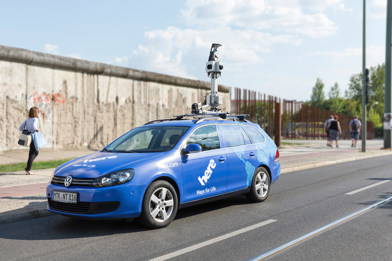
The mobile LIDAR system used by HERE.
Image © 2015 HERE
The significance of mobile LIDAR systems is that dense point clouds carrying geometric and photometric information of roads and their proximity are becoming available in unprecedented quality and quantity.
2.4. 3D warping and point-based rendering
3D warping and point-based rendering are two closely related image-based rendering techniques in that they both rely on a set of samples from the plenoptic function that carry depth information to synthesize images. Thus, they are a good fit for rendering with data acquired by mobile LIDAR systems.27 The conceptual difference between the two techniques is that 3D warping treats images as primitives,28 while point-based rendering uses points directly.
A straightforward approach to rendering with sample points carrying depth information is to simply reproject the points to form a new image. The problem with this approach is that the points are a discrete representation of a continuous domain and that will cause the synthesized image to have holes in it if the sample points are sparser than the resolution of the image.29 This is liable to happen, for example, if the viewpoint was moved closer to the objects.30 The solution lies in taking a signal processing approach to rendering where the sampled region of the plenoptic function is first reconstructed with a filter and then sampled again at a new viewpoint with increased resolution.31 Another approach involves forming a mesh from the sample points and interpolating color values across the warped mesh faces.32 Existing techniques either use the CPU or a forward mapping approach on the GPU to render frames.33
While important work has been conducted in the fields of 3D warping and point-based rendering, no solution to the problem at hand has been proposed – to the author’s best knowledge – that would be readily applicable in a web application. The solution presented in the next section was developed with the specific constraints of a web application in mind and takes a markedly different approach from existing techniques in that it is a backward mapping procedure that can be implemented on the GPU with no CPU overhead.
3. Perspective scaling
3.1. The goal
The goal of the research presented here was to develop a web application that allows continuous movement between immersive panoramas captured in the real world. As discussed in Section 1, this involves recovering frames between consecutive panoramas.
Given an immersive panorama at a point, an image looking in any direction can be found from that point. A method to recover frames along the [0, 0, 1]T vector in the camera's local coordinates will then allow for movement in all directions. Thus, the goal of this paper is defined as follows:
Given a digital image and its depth map, construct perspective-correct frames at locations displaced along the [0, 0, 1]T vector in the camera's local coordinates in real time in a web application.34

The green and orange cameras represent two immersive panoramas captured in the real world, while the blue camera represents a missing frame between the two.
3.2. Real time web application
Constructing frames in real time means that frames are rendered when they are required, thus allowing for arbitrary user interaction with confined space requirements. To render frames in real time at interactive rates, one needs the assistance of a graphical processing unit. The use of a GPU substantially constrains the implementation.
GPUs are in essence massively parallel matrix processing machines. The parallelism is why GPUs are so fast, but it also constrains applications in that the computation of a matrix element must be isolated from the computation of other elements. These constraints can be eased by sharing tasks between the CPU and the GPU, but the transfer of large data sets between the two comes with significant performance penalties. Real time rendering in a web application faces additional constraints, such as network bandwidth, low CPU performance and the sparse feature set of WebGL,35 the graphics API available in web browsers.
3.3. A digital image
A digital image can be thought of as a matrix of sample point and wave length pairs obtained by sampling regions of the plenoptic function visible to the camera. The sample points lie on an imaginary image plane and correspond to a perspective projection of the world. When the image is displayed, the function I that describes the wave lengths of light rays intersecting the image plane is reconstructed from the matrix.36
3.4. Perspective projection
Perspective projection gives answer to the question where rays of light that pass through the same point in space intersect some plane which is in essence how human vision and cameras work. The function that performs a perspective projection of a 3D point P to a plane perpendicular to the vector [0, 0, 1]T originating from the center of projection (COP) is:
PP(P) = (Px ⁄ Pz, Py ⁄ Pz), if Pz ≥ 1
The derivative of PP with respect to Pz is the following:
∂PP ⁄ ∂Pz = −1 ⁄ Pz2

Plot of the x, y = 1 slice of the PP function (red) and its derivative (blue) along the y and z axes.
The important characteristics of perspective projection for our purposes are the following:
- Objects farther from the COP appear smaller in the projection than objects closer.
- When moving the COP closer to an object, the closer the object, the faster it is growing in size.
- The farther away an object, the less the accuracy of depth values matters.
3.5. Displaced image
If the COP is displaced along the [0, 0, 1]T vector, the perspective projection at the displaced COP (COP′) can be expressed in terms of PP as follows:
PPD(A, z, Δz) = A · z ⁄ (z − Δz), if 0 < Δz < z,
where A is the perspective projection of P from the original COP, z is the z-coordinate of P and Δz is the magnitude of the displacement of the original COP.

The PPD function maps A to A′.
While constructing images by mapping points from the original image to the displaced one using the PPD function is straightforward in theory, it is challenging in practice. The only way to implement forward mapping with WebGL is to treat sample points as primitives and a high resolution image contains samples on the order of millions. To perform forward mapping, the dynamic buffering, decompression and representation of this data must be handled with JavaScript, in addition to the large amount of vertex processing required on the GPU and the complications involved with the reconstruction of the plenoptic function from a reprojection of sample points.37 In contrast, if images were produced by mapping sample points in the displaced image back to the original image using the inverse of PPD,38 these issues could be avoided. The backward mapping approach allows treating images as primitives,39 thus it requires minimal vertex processing40 and the reconstruction of the plenoptic function can be reduced to a texture mapping operation.
3.6. Displaced depth map
The challenge of constructing images using the inverse of PPD is that the depth map at COP′ needs to be known in advance to perform the mapping. Taking the same view of a depth map as of a digital image, it is a matrix of sample point and z-value pairs obtained from a 2D perspective projection of a 3D space. The function, DDM, that establishes the mapping between the original depth map, DM, and the displaced depth map at COP′ can be defined as follows:
DDM(A′, Δz) = DM(A′), if Δz = 0, or
DDM(A′, Δz) = DM(A′ ⁄ SF(DDM(A′, Δz − k), k)), if 0 < k ≤ Δz,
where A′ is the reprojection of a sample point in the original image, k is constant and the function SF (scale factor) is defined as follows:
SF(z, Δz) = z ⁄ (z − Δz), if 0 < Δz < z
To see why this formulation of DDM is useful, observe that:
1 < SF(z, Δz1) < SF(z, Δz2), if Δz1 < Δz2
Therefore, the values of a depth map at Δz can be found in a depth map at Δz − k in the same quadrant, but at a lesser distance from the origin.

The direction of displacement of the sample points.
To construct an image, the inverse of PPD is evaluated at sample points associated with pixels, so the values of DDM need to be produced only at these sample points. Since the reprojections of sample points will in general not map directly to sample points in the displaced image, the DDM function needs to be reconstructed from the reprojections to find the desired values.
Observe that k can be set to a value so small that upon the reconstruction of DDM with a box filter it is guaranteed that
DDM(D, Δz) = DDM(D + [±dh, ±dv]T, Δz − k), or
DDM(D, Δz) = DDM(D + [±dh, 0]T, Δz − k), or
DDM(D, Δz) = DDM(D + [0, ±dv]T, Δz − k), or
DDM(D, Δz) = DDM(D, Δz − k), where
D is a sample point in an image formed at COP′ and d is the horizontal or vertical distance between sample points. The sign of d depends on the quadrant of the image the sample point is located in. The value of DDM is then calculated by performing perspective projections with the three neighboring candidates and selecting the appropriate one if any.
![Visualization of the position of the points that are candidates for the value at D upon displacement of the <i>COP</i> by [0, 0, k]<sup>T</sup>.](./assets/images/dod-2.svg)
The depth map values at the points marked with green crosses are the candidates for the value at D upon the displacement of the COP by [0, 0, k]T.
Assuming without loss of generality that the horizontal dimension of the image is equal to or larger than its vertical dimension, the maximum value of k is given by the following inequality:
|Ax′ − Ax| < 2 ⁄ w,
where A is a sample point in the original image and A′ is its reprojection at a COP displaced by the vector [0, 0, k]T, while w is half the number of pixels in the horizontal dimension of the image. Expanding the terms and rearranging for k such that it satisfies the criterion for all points that are projected inside the image yields:41
k < 2 · zmin ⁄ (w · tan(θ) + 2),
where θ is half the horizontal field of view of the image.

The value of k must be small enough for the reprojection of a sample point A that contributes to the displaced image to remain in the green area (dashed line represents a non-inclusive endpoint).
While DDM lends itself to a recursive implementation following the observations above, displaced depth maps are produced with an iterative process: Since movement starts from a panorama where the value of Δz is 0, it makes sense to build depth maps iteratively as the movement progresses.42 This has one drawback: speed is confined to be a function of k.
3.7. Interpolation for increased resolution
The resolution of the sample points will become lower than the resolution of the synthesized image due to the displacement of the COP. To avoid artifacts in the constructed frames, the resolution of the sample points needs to be increased appropriately. This is achieved by a combination of two approaches: primitive geometric reconstruction is performed for depth maps and a bilinear filter is applied to images.
To increase the resolution of the coarse depth map yielded by the the DDM function, it is refined by perspective-correct barycentric interpolation. This means in practice that a sample point D in a displaced depth map is assumed to correspond to a point S on a triangle PQR in 3D. The perspective projection of PQR in turn corresponds to three sample points, ABC, in the original depth map.

The value of DDM at the sample point D is Pz. A refined value is acquired by assuming that D is the projection of a point S on the triangle PQR. The decrease in resolution is exhibited by the growing distance between the reprojections of sample points.
The three sample points are selected as follows: Let A be the position of the value at DDM(D, Δz) in the original depth map, and
B = A ± [dh, 0],
C = A ± [0, dv],
where d is the horizontal or vertical distance between sample points. The sign depends on the quadrant. To see why this works in most cases, consider the following:
It is known from the definition of DDM that
|D − O| ≤ |A′ − O|,
|B′ − O| < |D − O|,
|C′ − O| < |D − O|,
where O is the origin of the local coordinate system of the image, and the two closest points to A that are closer to the origin are B and C.
The fact that the surface of the sampled object is assumed to be planar between the points P, Q and R should not cause problems for the following reason: If the sampled object is close, then the area of the PQR triangle will be small and thus the depth values should not vary substantially. In contrast, if the sampled object is far away, then the area of the PQR triangle will be large, but in this case errors in depth values are tolerable as shown in Section 3.4. The method will break, however, if the points A, B and C sample different objects with large depth differences.
Using the refined depth map values, sample points in the current frame are mapped to the original image (as per Section 3.5) where the plenoptic function is reconstructed with a bilinear filter to render the desired image. A bilinear filter was chosen, because it is well-supported on GPUs by texture mapping.
3.8. The perspective scaling procedure
To summarize, the perspective scaling procedure consists of the following steps:
- Displace the COP by the [0, 0, k]T vector.
- Build the depth map at COP′ from the depth map at COP by selecting the appropriate value (if any) from the three neighboring candidates at each sample point.
- Refine this coarse depth map by perspective-correct barycentric interpolation.
- Map the sample points back to the original image using the refined depth values.
- Reconstruct the original image with a bilinear filter and sample it to construct the image at COP′.
- Repeat with COP′ as the COP.
The backward mapping procedure presented here can be implemented in a fragment shader and as a result it should be substantially faster than procedures that treat sample points as vertices or require computations on the CPU to generate frames.
4. Demo
A web application that implements perspective scaling to provide continuous movement between panoramas is presented along with this paper. The demo uses cubic projection panoramas that were captured in a synthetic scene created with the 3D graphics software, Blender. The depth maps were acquired by saving the depth buffer upon rendering the images. The scene consists of four streets in a downtown setting. A cone and a sphere were added to break Manhattan-world assumptions. The panoramas in one street capture two moving cars. The demo uses WebGL to render frames and was designed to run in the latest desktop Chrome and Firefox browsers.43 Care was not taken to optimize for efficiency.
The perspective scaling procedure is carried out at a steady 60 FPS at 512×512 resolution in the demo on modern laptops. A frame rate of 60 FPS was found to be maintained up to 1536×1536 resolution on a late 2013 MacBook Pro with integrated graphics.44 A drop in frame rate occurs upon changing input images, for two large textures are uploaded simultaneously to the GPU at this time. This could be avoided by optimizing the procedure.
Artifacts are present in the demo due to the disocclusion of objects: As the COP is displaced, parts of the scene may become visible that were previously blocked from view. Since there is no information about these parts of the scene in the original image, holes appear in the frames.

The disocclusion of an object caused by a change in viewpoint (top view).
While one can move continuously in the demo, transitions between panoramas are noticeable. This is caused by discrepancies between the frame recovered immediately before switching to the next panorama and the image from the next panorama. The discrepancies are caused by disocclusion artifacts and the difference in resolution of the sample points available to a frame recovered by perspective scaling and an original image.
5. Discussion
5.1. Real world application
As demonstrated, perspective scaling works well with panoramas taken in an artificial scene, but it is liable to perform worse with real world panoramas. One issue, already visible in the demo, is the presence of holes due to disocclusion. As real world scenes are a lot richer in detail than the demo, substantially more holes are likely to appear. A second issue is that real world scenes change while panoramas are captured: vehicles and pedestrians move around, lights change etc. This will make discrepancies between recovered and original images more apparent. Also, curvy streets, where there is no straight line on the road between two consecutive panoramas, can not be handled by perspective scaling in its current form.
5.2. Improvements
5.2.1. Using more data
While one panorama provides little information about the scenery, a collection of panoramas capture it reasonably well. Put another way, if some information is missing from one panorama, it is likely to be found in others.
Perspective scaling currently uses data only from the panorama being left behind. By extending the procedure, parts of a frame could be recovered from the following panorama.45 Thus, combining the two approaches, a higher quality reconstruction is possible. This would allow for avoiding many of the disocclusion artifacts and would provide smoother transitions between panoramas. The computational complexity of perspective scaling grows linearly with the number of sample points in time and space, so in theory this would amount to doubling the required computational resources. However, the resolution problem described in Section 3.7 does not apply to the next panorama, so the computationally expensive perspective-correct barycentric interpolation can be avoided in this case.
The frames produced by perspective scaling correspond to a perspective projection of the scene and can therefore be aligned with other perspective projections of it. For example, if an object in the scene is recovered by other means, a frame can be constructed by combining the results of perspective scaling and a separate perspective projection of that object.
In a real world application, most artifacts in a frame will be present over the region of the road, for it is usually littered with moving objects and it takes up a substantial part of the viewport during movement. These artifacts could be eliminated altogether if custom texture was generated for roads based on mapping data. Using such a custom texture might be even preferable to an exact reconstruction of the real world from a navigational point of view.
Using more data than what a single panorama offers will in general lead to higher quality frames and fewer holes.
5.2.2. Better solution to the resolution problem
No research was conducted to find the best solution to the resolution problem described in Section 3.7. The procedure presented to increase the resolution of depth maps suffers from three issues. The first is that it relies on assumptions untested in real world environments and produces artifacts if those assumptions break.46 The second is that the interpolation is carried out for every fragment of every frame, while the resolution problem occurs only for a subset of the fragments in a single frame. The third is that it misses improvements based on sensible assumptions about the scene such as handling the most common case of disocclusion when the occluded surface continues behind the occluder.47
Besides the best possible reconstruction, the ideal solution would require no preprocessing, would not add to the data load and could be implemented exclusively on the GPU. While the resolution problem is well researched, finding such a solution will prove to be challenging.
5.3. Comparison with other methods
Perspective scaling is a backward mapping 3D warping method that can be implemented exclusively on the GPU and is therefore feasible for use in real-time applications on platforms with low CPU performance such as web browsers and mobile devices. The data used by perspective scaling (panoramas and their depth maps) is easily segmentable and thus fit for delivery over the Internet. Using images as primitives for rendering provides performance gains over methods that use points as primitives, reduces the reconstruction of the plenoptic function to texture mapping and makes perspective scaling straightforward to implement in existing applications.
The artifacts described in Section 4 arise from the fact that perspective scaling relies on a discrete representation of the scene to render images. This is a problem inherent to all 3D warping and point-based rendering methods. The disadvantage of perspective scaling compared to these methods is that the speed of movement in the virtual environment is confined to be a function of k,48 and speeding up is possible only at the cost of performance.49
The advantage of perspective scaling (and 3D warping methods in general) compared to image-based rendering methods that use less geometric information50 is that it requires fewer samples from the plenoptic function and thus has lower storage requirements. Also, the frames generated by perspective scaling are guaranteed to correspond to a perspective projection of the scene. The disadvantage is that perspective scaling requires depth data, while these methods can render novel views based on images alone.
The advantage of perspective scaling compared to the traditional computer graphics approach is that it operates with the simplest geometric primitive (a point) and thus the challenging problem of geometric reconstruction is avoided. Furthermore, the computational complexity of perspective scaling is independent of the complexity of the scene. Yet the aforementioned artifacts do not occur with the traditional approach.
6. Conclusion
Perspective scaling in its current form is a suitable alternative to provide transitions between panoramas and with further research has the potential to achieve continuous movement in a virtual environment reconstructed from immersive panoramas.
7. Bibliography
E.H. Adelson and J.R. Bergen, "The Plenoptic Function and the Elements of Early Vision," in Computational models of visual processing. Cambridge, MA: MIT Press, 1991, pp. 3-20. Link.
J.F. Blinn, "What Is a Pixel?" IEEE Computer Graphics and Applications vol. 25, pp. 82-87, September 2005. Link.
A. Evans, "Web-Based Visualisation of On-Set Point Cloud Data," in Proceedings of the 11th European Conference on Visual Media Production, London, United Kingdom, 2014.
D.A. Forsyth and J. Ponce, Computer Vision: A Modern Approach, 2nd ed. Pearson, 2012.
M. Gross and H. Pfister, Eds., Point-Based Graphics. Morgan Kaufmann, 2007.
K. Ikeuchi, Ed., Computer Vision: A Reference Guide. Springer, 2014.
H. Kelly (2015, Feb. 17). "Nokia Is Paving the Way for Driverless Cars," CNN Money [Online]. Link. [Accessed: Apr. 29, 2015].
J. Lengyel, "The Convergence of Graphics and Vision." IEEE Computer vol. 31, pp. 46-53, May 1998. Link.
M. Levoy and P. Hanrahan, "Light Field Rendering," in Proceedings of the 23rd Annual Conference on Computer Graphics and Interactive Techniques, New Orleans, LA, 1996, pp. 31-42. Link.
W.R. Mark et al., "Post-Rendering 3D Warping," in Proceedings of the 1997 symposium on Interactive 3D graphics, Providence, RI, 1997, pp. 7-16. Link.
L. McMillan and G. Bishop, "Plenoptic Modeling: An Image-Based Rendering System," in Proceedings of the 22nd Annual Conference on Computer Graphics and Interactive Techniques, Los Angeles, CA, 1995, pp. 39-46. Link.
L. McMillan Jr., "An Image-Based Approach to Three-Dimensional Computer Graphics," Ph.D. dissertation, Dept. of Computer Science, Univ. North Carolina at Chapel Hill, 1997. Link.
M.J. Olsen et al., "Guidelines for the Use of Mobile LIDAR in Transportation Applications," Transportation Research Board, Washington, D.C., NCHRP Report 748, 2013. Link.
G. Poor (2015, Mar. 24). "Pssst! Our 'secret sauce' Is LiDAR," HERE 360 [Online]. Link. [Accessed: Apr. 29, 2015].
M. Schütz, "Rendering Large Point Clouds in Web Browsers," in Proceedings of CESCG 2015: The 19th Central European Seminar on Computer Graphics (non-peer-reviewed), Smolenice, Slovakia, 2015. Link.
S.M. Seitz and C.R. Dyer, "View Morphing," in Proceedings of the 23rd Annual Conference on Computer Graphics and Interactive Techniques, New Orleans, LA, 1996, pp. 21-30. Link.
J. Shade et al., "Layered Depth Images," in Proceedings of the 25th Annual Conference on Computer Graphics and Interactive Techniques, Orlando, FL, 1998, pp. 231-242. Link.
F. Shi et al., "On the Use of Ray-Tracing for Viewpoint Interpolation in Panoramic Imagery," in Computer and Robot Vision, 2009. CRV'09. Canadian Conference on, Kelowna, BC, 2009, pp. 200-207. Link.
H-Y. Shum et al., Image-Based Rendering. Springer, 2007.
A.R. Smith, "A Pixel Is Not A Little Square, A Pixel Is Not A Little Square, A Pixel Is Not A Little Square!," Microsoft Computer Graphics, Technical Memo 6, Jul. 17, 1995. Link.
R. Szeliski, Computer Vision: Algorithms and Applications. Draft, Sept. 3, 2010. Link.
C. Toth, "The New Era of Mobile Mapping Technology: Challenges and Trends in Sensing," Keynote, 2nd International Summer School on Mobile Mapping Technology, Tainan City, Taiwan, June 9-13, 2014 [Presentation slides]. Link.
8. Notes
- Such as zooming and interpolation or rendering the scene based on grossly simplified models.
- This line of thinking has been employed by McMillan before:
%cit P. 7. - An animation or an interactive application displays a sequence of images.
- %cit P. 1.
- %cit
- %cit
- %cit P. 392.
- Texture mapping is an exception which can be viewed as a precursor of IBR.
%cit P. 90. - %cit P. 399.
- %cit P. 2.
- %cit P. 11.
- %cit
- %cit Pp. 798-799.
- %cit P. 184.
- %cit P. 517.
- %cit P. 422.
- %cit P. 424.
- LIDAR stands for light detection and ranging.
- %cit Appendix A. p. 2.
- %cit P. 24.
- %cit Slide 85.
- %cit P. 33-35.
- It is unclear whether the accuracy reported is local or network accuracy. Furthermore, no data is provided on confidence levels or on the density of the samples which makes these numbers hard to evaluate.
- %cit
- %cit
- %cit Appendix B p. 31.
- %cit P. 5.
%cit P. 77. - %cit P. 1.
- %cit P. 248.
%cit P. 32. - %cit P. 78.
- %cit P. 52.
%cit P. 250. - %cit
%cit P. 54. -
The following 3D warping methods were examined:
- %cit
- %cit
- %cit
- %cit
- %cit
- splatting,
- GPU splatting,
- ray tracing of point models,
- rendering of very large point models and
- sequential point trees
%cit Pp. 247-339. - The displacement of the camera will increase the apparent size of objects visible at the original location, hence the name.
- For example, only vertex and fragment shaders are supported in WebGL, there is no straightforward way to blit a framebuffer and writing to multiple framebuffers is only possible using an ill-supported extension.
- For elaboration, see:
- %cit
- %cit
- For such a procedure, see splatting:
- %cit Pp. 247-293.
- %cit
- %cit
- PPD-1(D, z′, Δz) = D ⁄ [(z′ + Δz) ⁄ z′)], if 0 < Δz and 0 < z′, where D is a sample point in the displaced image and z′ is its associated depth map value.
- This means in practice that the data used for rendering is an image and its depth map that are uploaded to the GPU as textures.
- The vertex shader runs merely 24 times per frame in the demo.
- For a point to be projected inside the image it must satisfy the criterion, x ≤ z · tan(θ).
- Also, the GPU does not support recursion.
- Firefox 36.0.1 and Chrome 41.0.2272, precisely.
- MacBook Pro (Retina, 13-inch, Late 2013)
Processor: 2,4 GHz Intel Core i5
Memory: 8 GB 1600 MHz DDR3
Graphics: Intel Iris 1536 MB - The best way to go about this would be probably with layered depth images:%cit
- These artifacts are exhibited in the demo by the flickering effect sometimes present at the edge of buildings.
- As implemented in the compositing algorithm in Post-rendering 3D warping:
%cit - See Section 3.6 for elaboration.
- The performance penalty is not too bad in practice, because only the frequency of the execution of the relatively cheap DDM procedure needs to be increased in order to increase speed. For example, if an application targets 60 FPS, then the speed of movement is confined to 60 k/s, unless the DDM procedure is executed twice a frame, when the speed can be increased to 120 k/s and so on.
If the performance penalty is found to be prohibitive, speed can be increased at the cost of rendering quality. Potential approaches include downsampling the depth buffer and relaxing constraints on the epipolar region while setting the search range dynamically. - For example:
- %cit
- %cit